Team 5
Lab 3: Wall Following and Automatic Safety Controller
03/08/2019
Mitchell Guillaume
Daniel Wiest
Claire Traweek
Hector Castillo
Franklin Zhang
(Authored by Mitchell Guillaume)
Our team was tasked with implementing an autonomous wall following algorithm as well as an automatic safety stop feature for our robotic race car. This was our first time working with the physical car, so we began the lab by initializing teleop control and visualizing data in order to familiarize ourselves with the platform and the tools at our disposal. Both of our lab objectives rely on the car processing data from its Velodyne Puck lidar sensor and then calculating the desired steering angle and speed.
Our team organized our goals into two categories: hardware goals and software goals. Our two hardware goals were to drive the car manually in teleop mode and to use Rviz to render the car’s lidar data on our laptops, demonstrating our ability to perform critical tasks with the racecar platform. Our software goals were to implement a wall-following program and to implement an automatic stopping safety feature that overrides all other programs.
All of the hardware goals served to allow our team to become more familiar and comfortable with this expensive and complex platform. By taking time to master the basics, we’re more likely to have success in later projects when we set more challenging goals. The motivation for the software goals consists of two ideas. The first--safety--is simple. We don’t want the car to crash into anything, both to protect itself and its surroundings (including nearby people). The best way to ensure that the car will not crash is to have an automatic override that will stop the car in the case that it drives towards an obstacle. The wall follower serves as an example of a low level control scheme, in which control actions are calculated based on sensor data. While following a wall is relatively simple, it is again important to master the basics before moving into higher level robotic operations like path planning and semantic perception. With the wall follower, we hope to lay the foundation for a robust high-level architecture.
(Authored by Daniel Wiest)
The task of wall following necessitates an understanding of the environment external to the racecar. Because the contours of a given wall section are unique, it is important that the perception of the external surroundings provides sufficient information such that a robust control scheme can be developed. For this reason, our team’s exteroceptive sensing was performed by the Velodyne Puck lidar sensor, which reliably returns distance measurements within an error margin of 3 cm to points in all directions. This sensor is first rotated in software to account for the 60 degree mounting offset present on the vehicle, then used to construct an array of points with respect to the car’s coordinate frame.
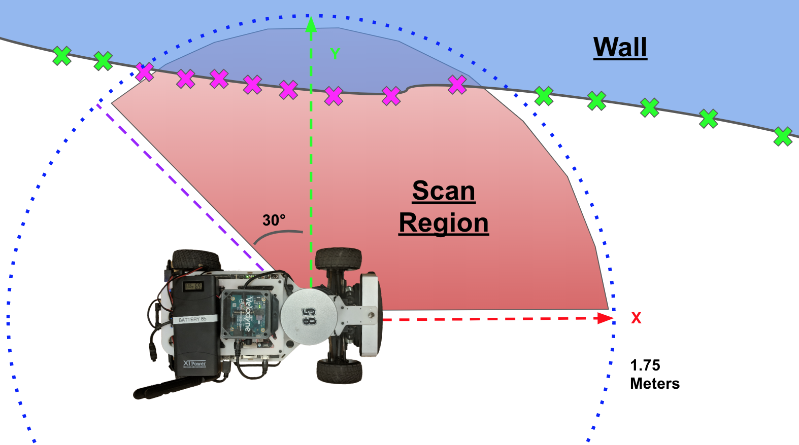
Next, the points are parsed by their relative location to the car, discarding all points lying outside of a 1.75 meter radius. This selection inherently constrains the largest distance from a wall that the vehicle can follow; however, this design choice was made after analyzing both the requirements stated for the performance of our vehicle as well as the car’s minimum turning radius. Intesting, our team determined that limiting the wall follower’s range further would prevent the car from detecting inside corners with enough time to respond, but expanding this range to greater distances caused the vehicle to react to objects not immediately important to its trajectory. This trial and error approach helped us determine our method for filtering.
Finally, points outside of the angles denoted by the “scan region” shown in Figure 1 are also discarded because they are not of relevance to following the line on a specific side. Once again, the specific values of these parameters were determined through experimental validation.
Figure 1. Scan Region Illustration – Only the points inside of the scan region pictured are used to find the wall position.
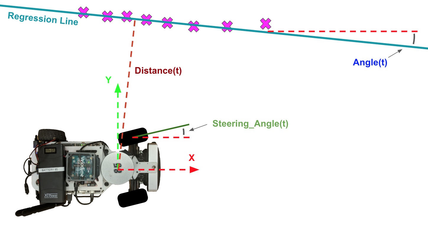
The algorithm performs a linear least-squares regression on the remaining points, which provides the coefficients that classify the approximate line describing the wall. Using these parameters, the angle between the car’s x-axis and the regression line as well as the perpendicular distance from the regression line to the car’s origin are calculated using the equations below. A graphical interpretation of these values are shown in Figure 2.
Where the equation for the line representing the wall is 


Figure 2. Line Regression – The points inside the scan region are regressed and then the distance between the car and the wall and the angle between the car and the wall are calculated.
A feedback controller uses these values to stabilize the vehicle. After consulting the notes from lecture, we implemented a controller that uses a combination of proportional and derivative terms. The controller operates on an error representing the distance between the robot and the setpoint. This term is then multiplied by the constant  and added to another term comprised of the angle between the car and the regression line multiplied by the constant
  . This value becomes the steering angle of the car as shown in the equations below, creating a closed-loop feedback system. Because this system is inherently nonlinear, it was linearized using the small angle approximation around zero degrees, so that
  . This simplified the system and made it analytically tractable. The values of and were first approximated then tuned experimentally. This process is discussed in greater detail in the experimental evaluation section of this report.


Our team chose to omit the integral component from our controller because the costs associated with this term outweighed the benefits as we observed in testing. The main drawback of this approach was that the summed error accumulated over time into very large values, causing large control inputs that resulted in erratic behavior known as integral windup. Additionally, the integral term resulted in greater overshoot in the response of the car with respect to the metric discussed in the experimental evaluation section. For these reasons, an integral component was not included in our controller.
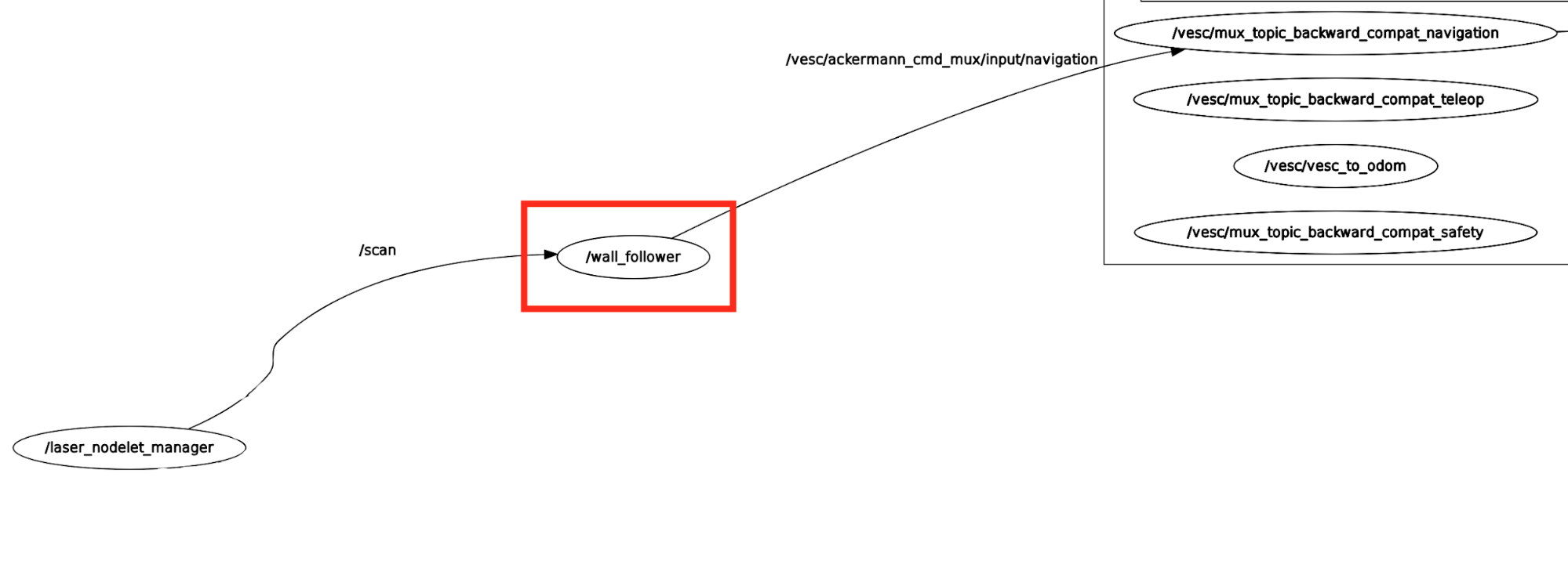
The wall follower consists of a single node which subscribes to the points returned by the Velodyne lidar on the “/scan” topic. Because the velodyne lidar is rotated approximately 60 degrees out of alignment with the car’s forward axis, the array representing these points is manipulated such that the resulting coordinates are aligned with the robot chassis. Next, after performing the operations described in Section 2.1.1, the steering angle command is calculated and then published to the “/vesc/ackermann_cmd_mux/input/navigation” topic.
Figure 3. rqt_graph Node Map – This figure illustrates the interconnections with the wall_follower node.
(Authored by Franklin Zhang)
The safety controller takes uses lidar data and the published drive commands and puts this information into an algorithm that decides whether to overwrite the current drive command or not. The algorithm predicts the future position of the car and stops the car if that predicted distance is below a minimum threshold.

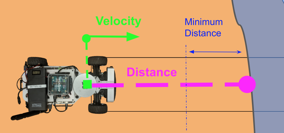
The problem was first simplified into one-dimension. The two-dimensional lidar data (range, angle), is converted into cartesian coordinates centered at the lidar, where the x axis points towards the front of the robot and the y axis points to the left. The lidar points that aren’t directly in front of the car are filtered out. The car has a base length of approximately .2 meters, so only the data points where -0.15 < x < 0.15 were considered. From the filtered dataset, the point with the smallest y coordinate is then passed into the next step of the algorithm. At this step, the system is a one-dimensional problem where we only consider the movement of the car in the x direction. This implementation does not consider steering angle which is traded off for simplicity.
Figure 4. Stopping Distance Calculation – The robot retrieves the closest point from a filtered lidar dataset to measure distance to the nearest obstacle. The current distance and velocity are used to predict if the car will get too close to an obstacle in the next time step, in which case the controller stops the car.
With the current position and velocity data, we can estimate the position of the car in the next time step. More precisely, we can use the equation

where  is the distance from the wall to the lidar,
  is the current velocity command, and
  is the time between each iteration. A minimum distance is set, so that when
  is less than that minimum distance, the safety controller publishes a new drive command with a velocity set to 0 which overwrites the existing command.
With the current implementation, the distance  when the safety controller would be triggered has a linear relationship with the robot velocity. In reality, the relationship between these two factors isn’t linear. Assuming a constant braking force, the distance required to stop the car given the velocity is related to the square of the velocity. Even this model might not be accurate enough to describe the system because it ignores other physical factors. We can assume that the distance that the vehicle would need to is greater with greater velocity. We can tune the weight of the velocity term. A safety factor
  was added to the existing equation like so:

Through experimentation, we can figure out a value of that works to stop our car within a range of speeds at which our robot will operate.
The velodyne lidar that we are using has a minimum range of . The safety controller needed to account for this, because if any objects were to violate this minimum range, the robot would lose sight of it. Thus, the minimum distance from the wall was chosen based on this lower bound.
(Authored by Claire Traweek)
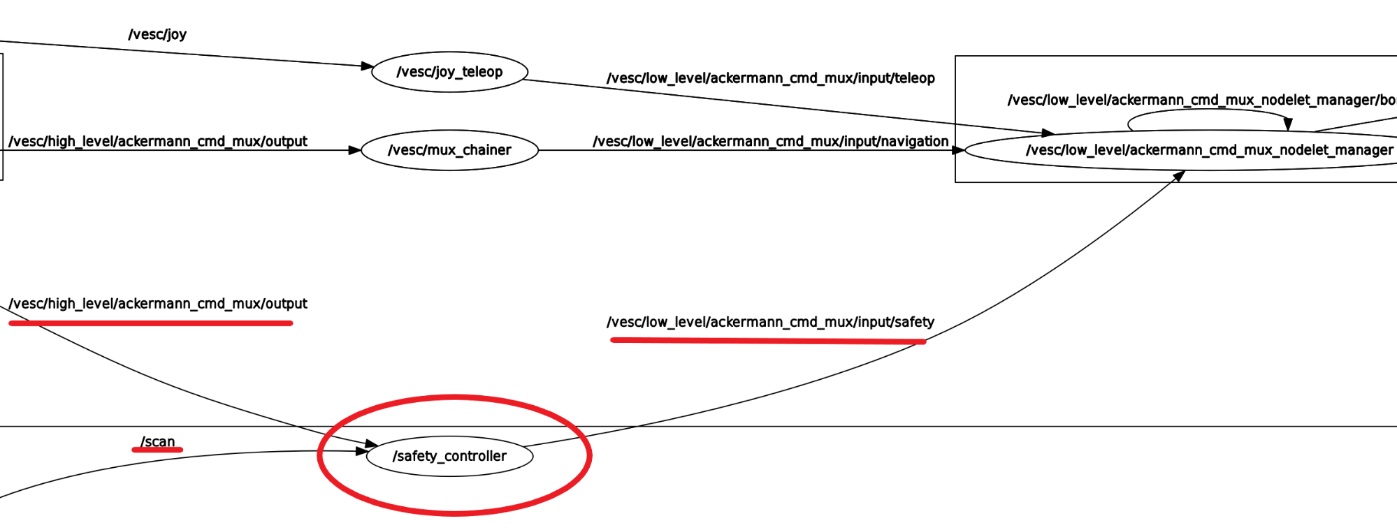
The safety controller is contained in a node called “safety_controller.py” inside of the safety_controller package. This node listens to the output of the high level command mux (the /vesc/high_lecel/ackermann_cmd_mux). Its output is the second highest priority input to the low level command mux, the last mux before the command is sent to the car. This way, the safety controller overrides
any code coming directly from the high level mux, but is itself overridden by teleop control. This setup is shown in Figure 5. The node called “drive.py” inside of the safety_controller package was used to drive the robot forward at varying speeds for testing purposes.
Figure 5: rqt_graph safety - The safety controller subscribes to the /scan and /vesc/high/level/ackermann_cmd/out to get lidar scan data and drive commands respectively. It publishes to /vesc/low_level/ackermann_cmd_mux/input/safety.
(Authored by Daniel Wiest)
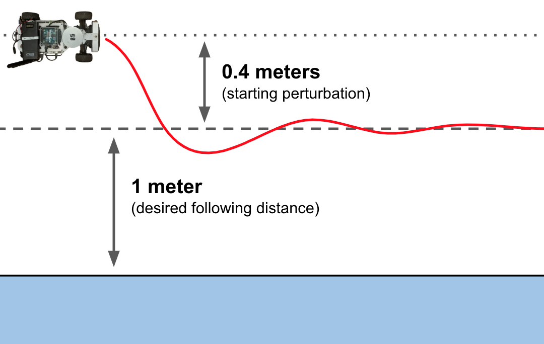
The large amount of experimental trial and adjustment required to fine tune the controller gains necessitated the development of a metric with which to establish the relative success of a set of parameters. In response to this need, our team experimentally verified our solution by setting the car 1.4 meters from the wall as shown in Figure 6, then releasing it parallel to a straight section of wall with a desired distance of 1 meter.
Figure 6. Disturbance Recovery Test Setup – The car begins 0.4 meters from its desired tracking distance and then the distance between the actual and desired offsets to the wall is recorded in time at 0.5 meters per second to permit the quantitative comparison of different responses.
By tracking the error between the car and its setpoint, we were able to make a quantitative assessment of the modifications made. Figure 7 and Figure 8 illustrate the evolution of the difference between the actual distance to the wall and the desired distance to the wall over time. Figure 7 illustrates the response achieved near the beginning of tuning, and Figure 8 shows the results achieved after successfully tuning the values of the proportional and derivative terms. Of particular note, the amount of time required to reach 2% of the initial disturbance value reduced from around 5.5 seconds to approximately 2.6 seconds after experimental tuning.
Figure 7. Controller Parameter Tuning – This graph shows the distance error with respect to the setpoint in time before the controller gains and were adjusted.
Figure 8. Controller Parameter Tuning – This graph shows this same quantity for the system with  and
and  . This optimized response reaches 2% of its initial value almost three seconds faster than the unoptimized response.
(Authored by Franklin Zhang)
The minimum distance and safety factor parameter was selected experimentally. We settled on the values of .6 meters for the minimum distance and 5 for the safety factor based on the visual assessment of the performance and consistency across varying speeds. In order to quantify the performance of the safety controller, we ran some tests where we drove the robot toward a wall at varying speeds, relying on the safety controller to stop the car. These tests were performed with velocities ranging between 0 and 3 meters per second and the stopped distance between the car and the wall was recorded. The results of this tests are shown in Figure 9.
Figure 9. Safety Controller Evaluation - With the minimum distance set to .6 meters and safety factor set to 5, the safety controller was tested by running the car into a wall at varying speeds and allowing the safety controller to stop the car. The car’s stopped distance from the wall was recorded. The car stops at around .8 meters from the wall when the velocity ranges from 0 to 3.
The results from the test are promising because they show that the safety controller is able to make the robot consistently stop at the same distance from the wall at varying velocities. This stopped distance can be tuned by changing the minimum distance parameter in the algorithm. The safety controller can be easily adjusted and tested for future use cases using these tuning parameters.
(Authored by Hector Castillo)
This lab was very significant in terms of learning. This was our first lab working together as a team, using our robot, and preparing a briefing. While we are constantly learning new technical knowledge and skills, we found that most of our learning happened with regards to our team organization and intercommunication.
One of the first steps of this lab was to take working wall-following code proven in simulation and apply it to the real-world car. We quickly learned that what works in simulation does not necessarily work on real-life hardware. We were able to overcome this by taking the woking framework and adjusting the and parameters to the new platform through empirical testing as mentioned in Section 3.1.
We also learned that there are tradeoffs between robustness, complexity, and implementation time. When creating our safety controller, we traded some robustness and computational intensity for a simpler solution that took less time to implement. However, we later wrote an additional, more robust yet computationally intensive safety controller that accounts for the steering angle. We may implement this new controller if we find that our current controller does not meet our requirements.
Organization is important when tackling any challenge, especially when working in a team. We learned many important things in team organization and communication such as setting goals, creating success metrics, and setting a defined meeting structure. We also want to ensure that everyone’s tasks are clearly defined in order to help with subsystem integration.
This was also our first time giving a briefing as a team. Overall, our briefing went swimmingly, and we received some great feedback. Some of this feedback included adding slide numbers, having a more descriptive presentation title, being aware of colors that look the same in grayscale, being careful with terminology, providing motivation and explanation for equations used, and creating team branding.
(Authored by Claire Traweek)
In the future, should the safety controller prove too erratic, we have an alternative, more computationally intensive version of the code that predicts if the car needs to break based on the direction the car is turning, not the direction the car is currently facing. If the robot needs to make a lot of sudden, fast turns, this system would be beneficial. Another improvement for the safety controller is forced deceleration as the robot approaches a wall. In addition to eliminating some of the jerky movement that puts wear on the car, such a system could allow us to get closer to the wall with greater accuracy.
Further experimentation with  values would improve our wall follower, as would the eventual implementation of the
  component. The wall follower could also be further specialized for narrow corridors with more specific filtering. Additionally, selectively slowing the speed of the robot as it navigates corners would tighten the error that occurs around tight corners.
Finally, we want to create some branding for our team such as a team name, a logo, and a nice color palette. Doing so will help establish our identity within RSS, liven up our website and presentation slides, and further unify us as a team.
This document was revised and edited by Hector Castillo and Claire Traweek.